tanggle: Visualization of phylogenetic networks in a ggplot2 framework

Klaus Schliep

Graz University of Technology

Marta Vidal-García

University of Calgary

Leann Biancani

University of Rhode Island

Francisco Henao Diaz

University of British Columbia

Eren Ada

University of Rhode Island

Claudia Solís-Lemus

University of Wisconsin-Madison
klaus.schliep@gmail.com

Source: vignettes/tanggle_vignette.Rmd

tanggle_vignette.Rmd

Introduction

Here we present a vignette for the R package tanggle, and provide an overview of its functions and their usage. Tanggle extends the ggtree R package (Yu et al. 2017) to allow for the visualization of several types of phylogenetic networks using the ggplot2 (Wickham 2016) syntax. More specifically, tanggle contains functions to allow the user to effectively plot: (1) split (i.e. implicit) networks (unrooted, undirected) and (2) explicit networks (rooted, directed) with reticulations. It offers an alternative to the plot functions already available in ape (Paradis and Schliep 2018) and phangorn (Schliep 2011).

List of functions

Function name	Brief description
`geom_splitnet`	Adds a splitnet layer to a ggplot, to combine visualising data and the network
`ggevonet`	Plots an explicit network from a phylo object
`ggsplitnet`	Plots an implicit network from a phylo object
`minimize_overlap`	Reduces the number of reticulation lines crossing over in the plot
`node_depth_evonet`	Returns the depths or heights of nodes and tips in the phylogenetic network

Getting started

Install the package from Bioconductor directly:

if (!requireNamespace("BiocManager", quietly = TRUE))
    install.packages("BiocManager")

BiocManager::install("tanggle")

Or install the development version of the package from Github.

if (!requireNamespace("remotes", quietly=TRUE))
  install.packages("remotes")
remotes::install_github("KlausVigo/tanggle")

If you need to install ggtree from github:

remotes::install_github("YuLab-SMU/ggtree")

And load all the libraries:

library(tanggle)
library(phangorn)
library(ggtree)

Split Networks

Split networks are data-display objects which allow for the definition of 2 (or more) options for non-compatible splits. Split networks are most often used to visualize consensus networks (Holland et al. 2004) or neighbor-nets (Bryant and Moulton 2004). This can be done either by using the consensusNet or neighbor-net functions in phangorn (Schliep 2011) or by importing nexus files from SplitsTree (Huson and Bryant 2006).

Data Types

tanggle accepts three forms of input data for split networks. The following input options all generate a networx object for plotting.

Nexus file created with SplitsTree (Huson and Bryant 2006) and read with the read.nexus.network function in phangorn (Schliep 2011).
Read in a split network in nexus format:

fdir <- system.file("extdata/trees", package = "phangorn")
Nnet <- phangorn::read.nexus.networx(file.path(fdir,"woodmouse.nxs"))

A collection of gene trees (e.g.~from RAxML (Stamatakis 2014)) in one of the following formats:
- Nexus file read with the function read.nexus
- Text file in Newick format (one gene tree per line) read with the function read.tree A consensus split network is then computed using the function consensusNet in phangorn (Schliep 2011).

Sequences in nexus, fasta or phylip format, read with the function read.phyDat in phangorn (Schliep 2011) or the function read.dna in ape (Paradis and Schliep 2018). Distances matrices are then computed for specific models of evolution using the function dist.ml in phangorn (Schliep 2011) or dist.dna in ape (Paradis and Schliep 2018). From the distance matrix, a split network is reconstructed using the function neighborNet in phangorn (Schliep 2011). Optional: branch lengths may be estimated using the function splitsNetworks in phangorn (Schliep 2011).

Plotting a Split Network:

We can plot the network with the default options:

p <- ggsplitnet(Nnet) + geom_tiplab2()
p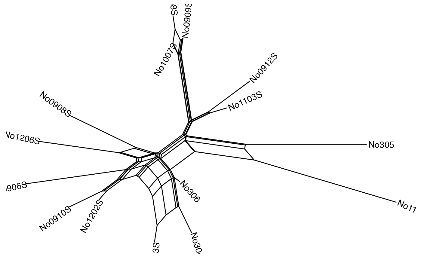

When we can set the limits for the x and y axis so that the labels are readable.

p <- p + xlim(-0.019, .003) + ylim(-.01,.012) 
p

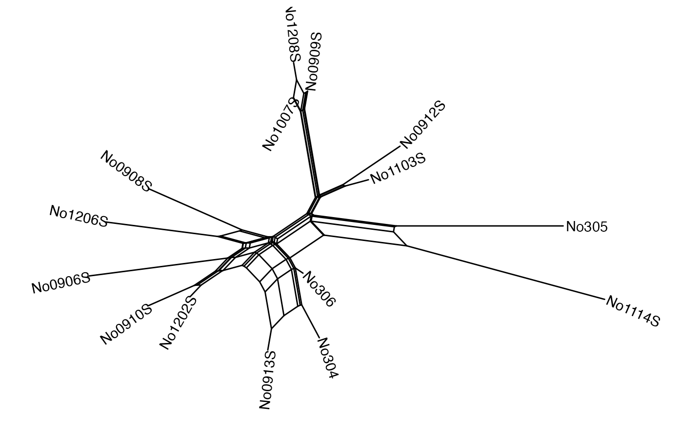
You can rename tip labels. Here we changed the names to species from 1 to 15:

Nnet$translate$label <- seq_along(Nnet$tip.label)

We can include the tip labels with geom_tiplab2, and customize some of the options. For example, here the tip labels are in blue and both in bold and italics, and we show the internal nodes in green:

ggsplitnet(Nnet) + geom_tiplab2(col = "blue", font = 4, hjust = -0.15) + 
    geom_nodepoint(col = "green", size = 0.25)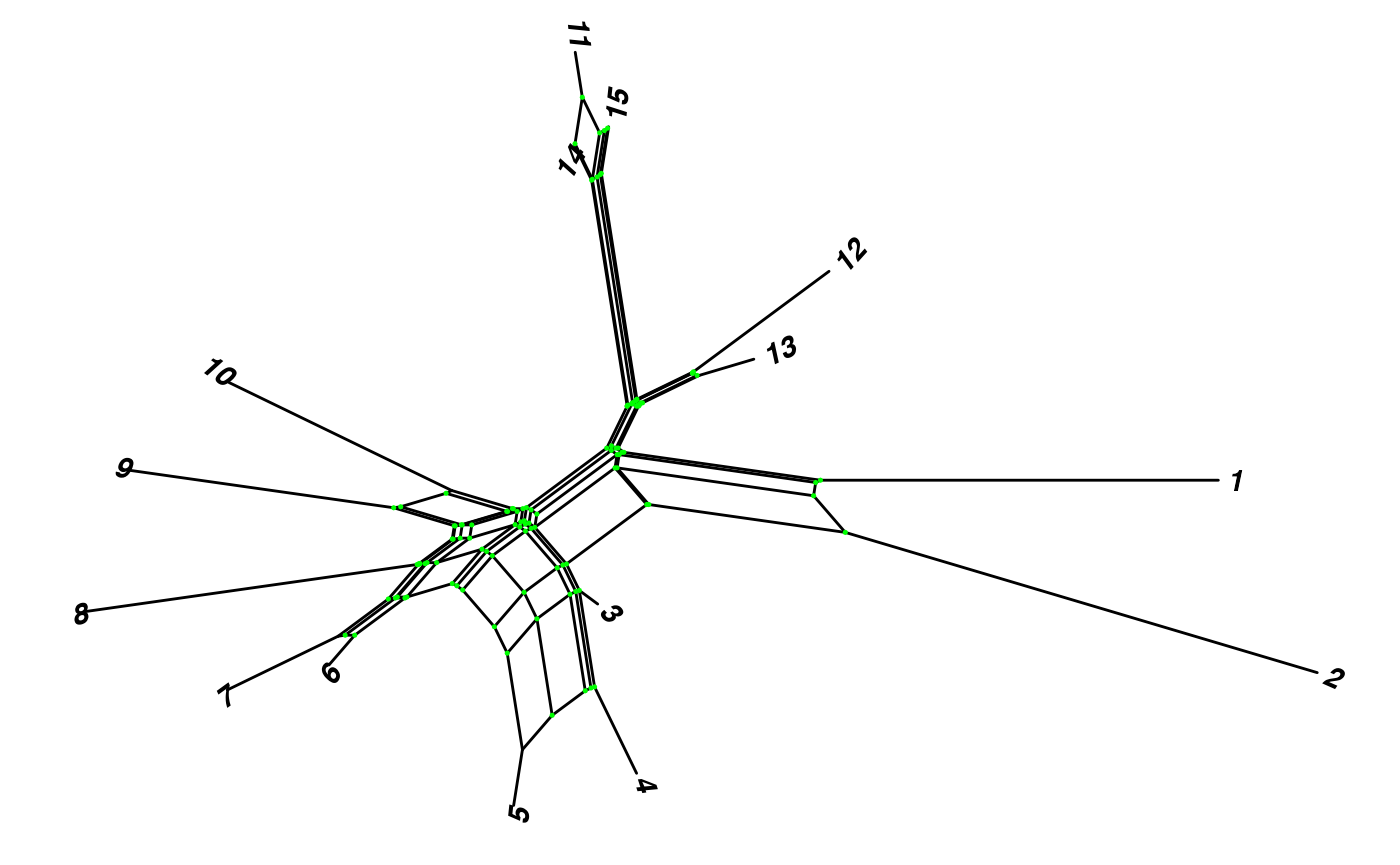

Nodes can also be annotated with geom_point.

ggsplitnet(Nnet) + geom_point(aes(shape=isTip, color=isTip), size=2)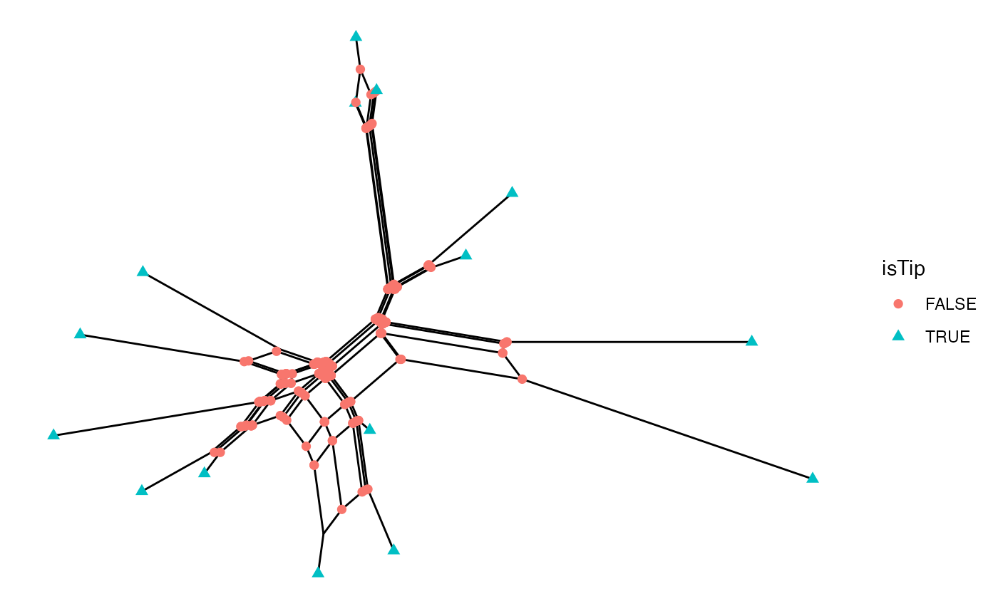

Plotting Explicit Networks

The function ggevonet plots explicit networks (phylogenetic trees with reticulations). A recent addition to ape (Paradis and Schliep 2018) made it possible to read in trees in extended newick format (Cardona, Rosselló, and Valiente 2008).

Read in an explicit network (example from Fig. 2 in Cardona et al. 2008):

z <- read.evonet(text = "((1,((2,(3,(4)Y#H1)g)e,(((Y#H1,5)h,6)f)X#H2)c)a,
                 ((X#H2,7)d,8)b)r;")

Plot an explicit network:

ggevonet(z, layout = "rectangular") + geom_tiplab() + geom_nodelab()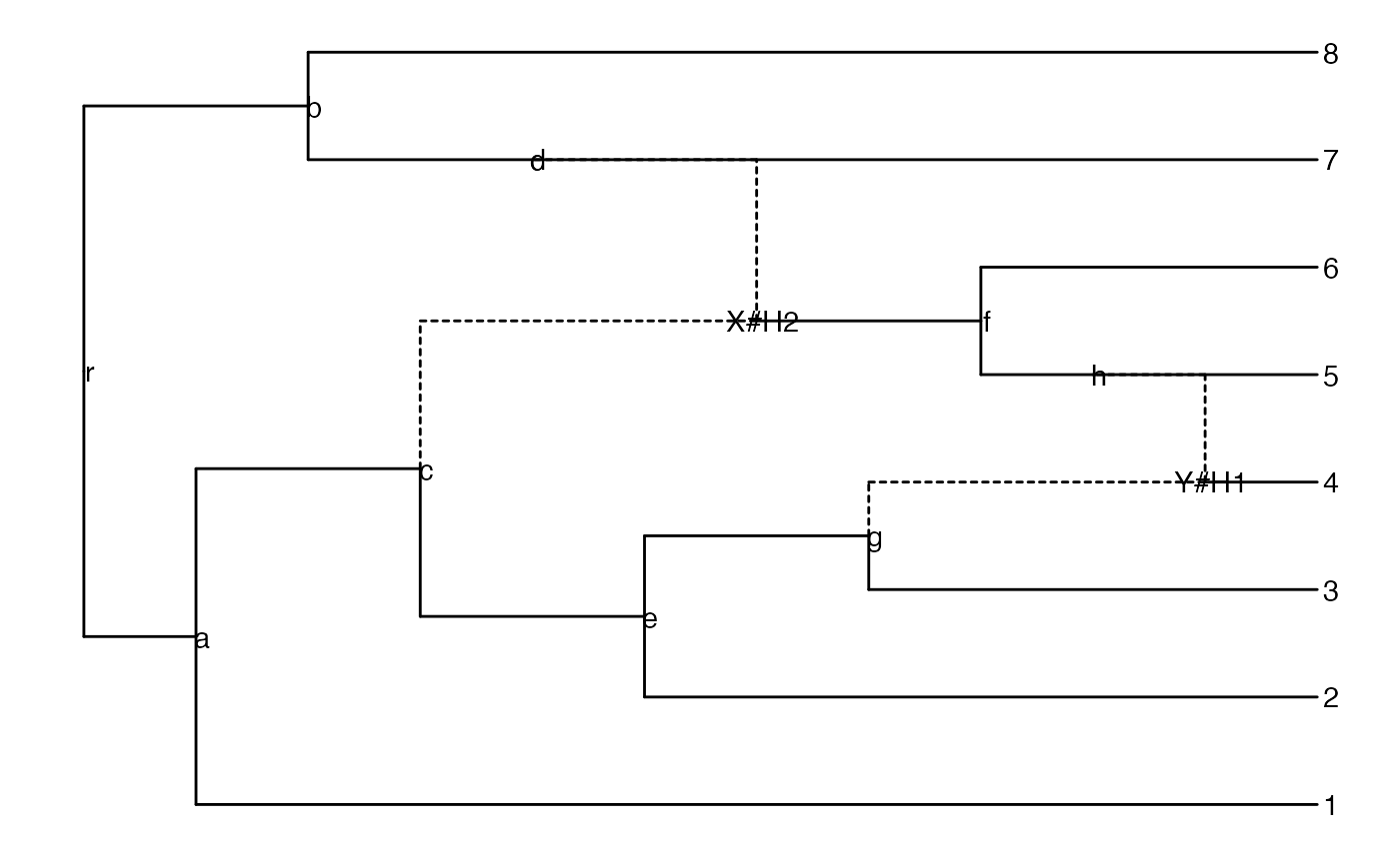

p <- ggevonet(z, layout = "slanted") + geom_tiplab() + geom_nodelab()
p + geom_tiplab(size=3, color="purple")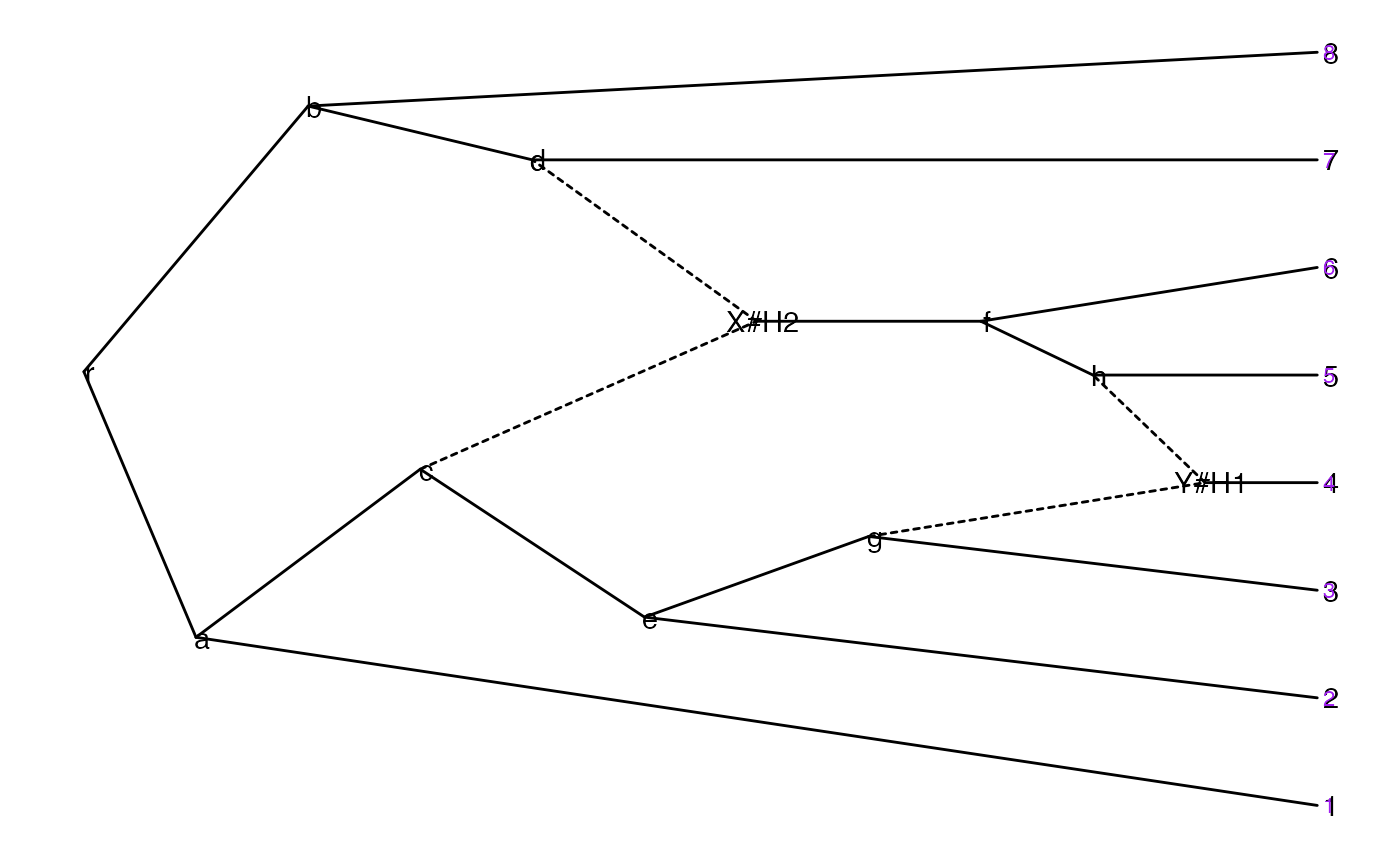

p + geom_nodepoint(color="#b5e521", alpha=1/4, size=10)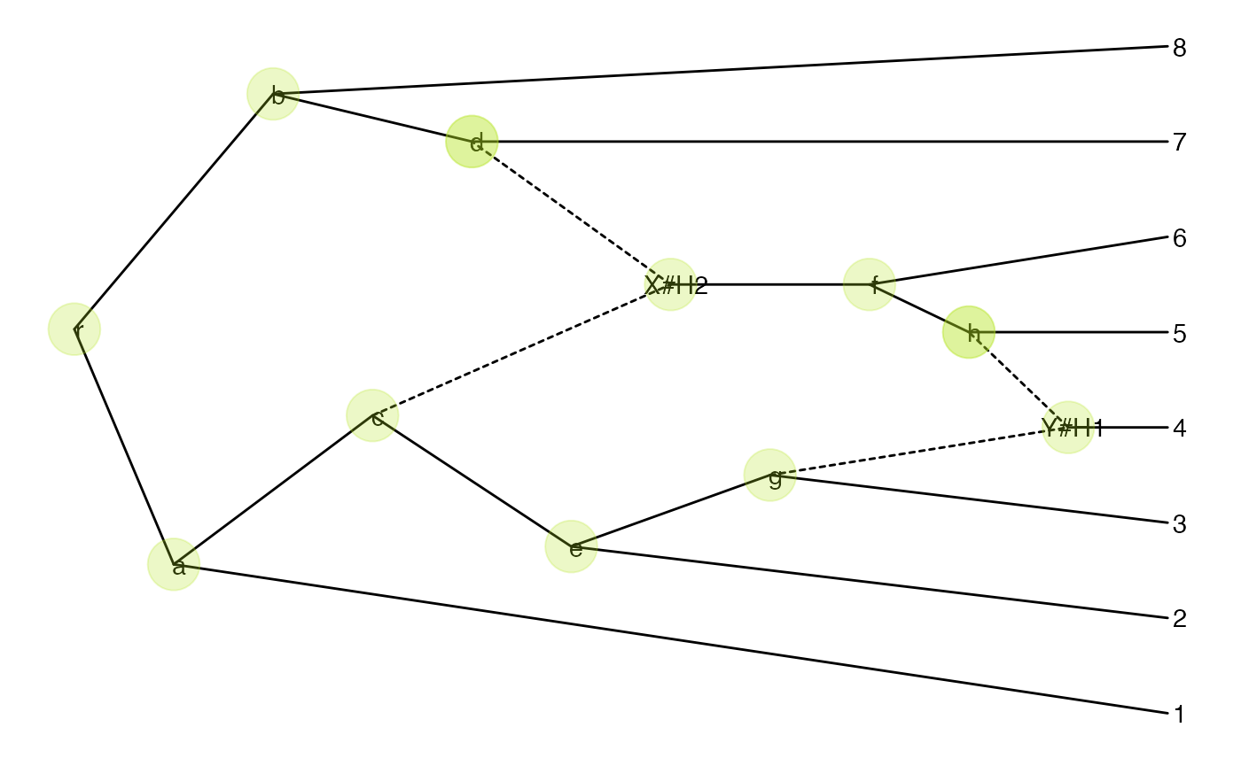

Summary

This vignette illustrates all the functions in the R package tanggle, and provides some examples on how to plot both explicit and implicit networks. The split network plots should take most of the functions compatible with unrooted trees in ggtree. The layout options for explicit network plots are rectangular or slanted.

Session info

sessionInfo()
#> R version 4.1.1 (2021-08-10)
#> Platform: x86_64-apple-darwin17.0 (64-bit)
#> Running under: macOS Catalina 10.15.7
#> 
#> Matrix products: default
#> BLAS:   /Library/Frameworks/R.framework/Versions/4.1/Resources/lib/libRblas.0.dylib
#> LAPACK: /Library/Frameworks/R.framework/Versions/4.1/Resources/lib/libRlapack.dylib
#> 
#> locale:
#> [1] en_US.UTF-8/en_US.UTF-8/en_US.UTF-8/C/en_US.UTF-8/en_US.UTF-8
#> 
#> attached base packages:
#> [1] stats     graphics  grDevices utils     datasets  methods   base     
#> 
#> other attached packages:
#> [1] phangorn_2.7.1   ape_5.5          tanggle_0.99.2   ggtree_3.0.4    
#> [5] ggplot2_3.3.5    BiocStyle_2.20.2
#> 
#> loaded via a namespace (and not attached):
#>  [1] Rcpp_1.0.7          lattice_0.20-44     tidyr_1.1.3        
#>  [4] rprojroot_2.0.2     digest_0.6.27       utf8_1.2.2         
#>  [7] R6_2.5.1            evaluate_0.14       highr_0.9          
#> [10] pillar_1.6.2        ggfun_0.0.3         yulab.utils_0.0.2  
#> [13] rlang_0.4.11        lazyeval_0.2.2      Matrix_1.3-4       
#> [16] rmarkdown_2.10      pkgdown_1.6.1       labeling_0.4.2     
#> [19] textshaping_0.3.5   desc_1.3.0          stringr_1.4.0      
#> [22] igraph_1.2.6        munsell_0.5.0       compiler_4.1.1     
#> [25] xfun_0.25           pkgconfig_2.0.3     systemfonts_1.0.2  
#> [28] gridGraphics_0.5-1  htmltools_0.5.2     tidyselect_1.1.1   
#> [31] tibble_3.1.4        bookdown_0.24       codetools_0.2-18   
#> [34] quadprog_1.5-8      fansi_0.5.0         crayon_1.4.1       
#> [37] dplyr_1.0.7         withr_2.4.2         grid_4.1.1         
#> [40] nlme_3.1-152        jsonlite_1.7.2      gtable_0.3.0       
#> [43] lifecycle_1.0.0     magrittr_2.0.1      scales_1.1.1       
#> [46] tidytree_0.3.4      stringi_1.7.4       cachem_1.0.6       
#> [49] farver_2.1.0        fs_1.5.0            ellipsis_0.3.2     
#> [52] ragg_1.1.3          generics_0.1.0      vctrs_0.3.8        
#> [55] fastmatch_1.1-3     tools_4.1.1         treeio_1.16.2      
#> [58] ggplotify_0.1.0     glue_1.4.2          purrr_0.3.4        
#> [61] parallel_4.1.1      fastmap_1.1.0       yaml_2.2.1         
#> [64] colorspace_2.0-2    BiocManager_1.30.16 aplot_0.1.0        
#> [67] memoise_2.0.0       knitr_1.33          patchwork_1.1.1

References

Bryant, David, and Vincent Moulton. 2004. “Neighbor-Net: An Agglomerative Method for the Construction of Phylogenetic Networks.” Molecular Biology and Evolution 21 (2): 255–65. https://doi.org/10.1093/molbev/msh018.

Cardona, Gabriel, Francesc Rosselló, and Gabriel Valiente. 2008. “Extended Newick: It Is Time for a Standard Representation of Phylogenetic Networks.” BMC Bioinformatics 9 (1): 532. https://doi.org/10.1186/1471-2105-9-532.

Holland, Barbara R., Katharina T. Huber, Vincent Moulton, and Peter J. Lockhart. 2004. “Using Consensus Networks to Visualize Contradictory Evidence for Species Phylogeny.” Molecular Biology and Evolution 21 (7): 1459–61. https://doi.org/10.1093/molbev/msh145.

Huson, D. H., and D. Bryant. 2006. “Application of Phylogenetic Networks in Evolutionary Studies.” Molecular Biology and Evolution 23 (2): 254–67.

Paradis, Emmanuel, and Klaus Schliep. 2018. “Ape 5.0: An Environment for Modern Phylogenetics and Evolutionary Analyses in R.” Bioinformatics 35 (3): 526–28.

Schliep, Klaus Peter. 2011. “Phangorn: Phylogenetic Analysis in R.” Bioinformatics 27 (4): 592–93. https://doi.org/10.1093/bioinformatics/btq706.

Stamatakis, A. 2014. “raXml Version 8: A Tool for Phylogenetic Analysis and Post-Analysis of Large Phylogenies.” Bioinformatics 30 (9): 1312–3.

Wickham, Hadley. 2016. Ggplot2: Elegant Graphics for Data Analysis. Springer-Verlag New York. https://ggplot2.tidyverse.org.

Yu, Guangchuang, David Smith, Huachen Zhu, Yi Guan, and Tommy Tsan-Yuk Lam. 2017. “Ggtree: An R Package for Visualization and Annotation of Phylogenetic Trees with Their Covariates and Other Associated Data.” Methods in Ecology and Evolution 8 (1): 28–36. https://doi.org/10.1111/2041-210X.12628.