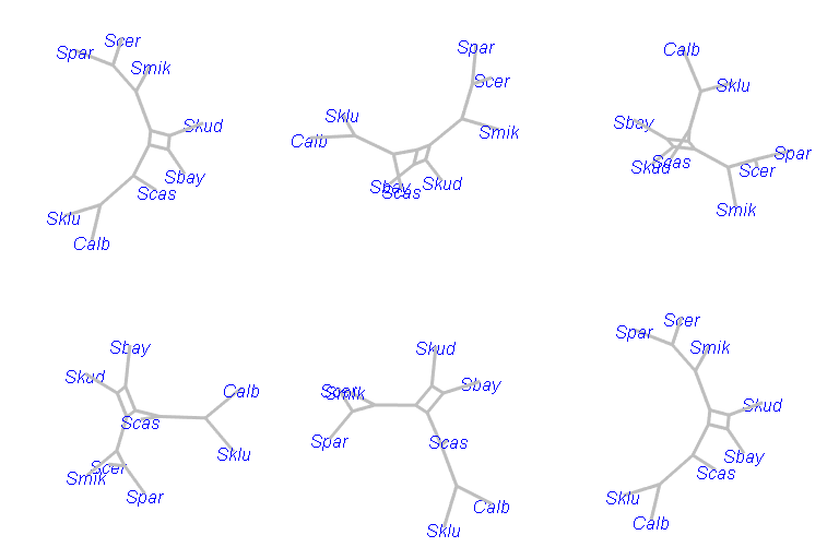
This tutorial gives a basic introduction for constructing
phylogenetic networks and adding parameters to trees or networx objects
using phangorn
(Schliep 2011) in R. Splits graphs or
phylogenetic networks are a useful way to display conflicting data or to
summarize different trees. Here, we present two popular networks,
consensus networks (Holland et al. 2004)
and Neighbor-Net (Bryant and Moulton 2004; Bryant
and Huson 2023).
Trees or networks are often missing either edge weights or edge support
values. We show how to improve a tree/networx object by adding support
values or estimating edge weights using non-negative Least-Squares
(nnls).
We first load the phangorn package and a few data sets we use in this vignette.
## Loading required package: apeconsensusNet
A consensusNet (Holland et al. 2004) is a generalization of a consensus tree. Instead of only representing splits (taxon bipartitions) occurring in at least 50% of the trees in a bootstrap or MCMC sample one can use a lower threshold and explore competing splits. Note that, in its basic implementation used here, the consensusNet edge lengths are proportional to the frequency of the corresponding splits in the provided list of trees.
The input for consensusNet is a list of trees i.e. an
object of class multiPhylo.
set.seed(1)
bs <- bootstrap.phyDat(yeast, FUN = function(x)nj(dist.hamming(x)),
    bs=100)
tree <- nj(dist.hamming(yeast))
cnet <- consensusNet(bs, .3)
par("mar" = rep(1, 4), "mfrow"=c(1,2))
tree <- plotBS(midpoint(tree), bs, "phylogram", main="a)")
plot(cnet, show.edge.label=TRUE, main="b)")
Tree with bootstrap values and consensusNet for the same trees
In many cases, consensusNet will return more than two
incompatible (competing) splits. This cannot be plotted as a planar
(2-dimensional) graph. Such as situation requires a n-dimensional graph,
where the maximum number of dimensions equals the maximum number of
incompatible splits. For example, if we have three alternative
incompatible splits: (A,B)|(C,D) vs. (A,C)|(B,D) vs. (A,D)|(B,C), we
need a 3-dimensional graph to show all three alternatives. A nice way to
get still a good impression of the network is to plot it in 3D.
plot(cnet, "3D")
# rotate 3d plot
play3d(spin3d(axis=c(0,1,0), rpm=6), duration=10)
# create animated gif file
movie3d(spin3d(axis=c(0,1,0), rpm=6), duration=10)
which will result in a spinning graph similar to this

The rendering of the networx is done using the the
fantastic igraph package (Csardi and Nepusz
2006).
neighborNet
The function neighborNet implements the popular method
of Bryant and Moulton (2004). The
Neighbor-Net algorithm is essentially a 2D-version of the Neighbor
joining algorithm. The Neighbour-net is computed in two steps: the first
computes a circular ordering of the taxa in the data set; the second
step involves the estimation of edge weights using non-negative
Least-Squares (nnls).
dm <- dist.hamming(yeast)
nnet <- neighborNet(dm)
The advantage of Neighbor-Net is that it returns always a circular split system which can be always displayed in a planar (2D) graph. For planar graphs we can also plot only the outline (Bagci et al. (2021)) as in figure @ref(fig:outline) c).
par("mar" = rep(1, 4), "mfrow" = c(1, 3))
plot(nnet, main="a)")
plot(nnet, main="b)", use.edge.length = FALSE)
plot(nnet, type = "outline", main="c)", use.edge.length = FALSE)
NeighborNet showing a) all edges, without using edge length information b) and only the outline c).
Adding support values
We can use the generic function addConfidences to add
(branch) support values from a tree, i.e. an object of class
phylo to a networx, splits or
phylo object. The Neighbor-Net object we computed above
provides no support values. We can add the support values from the tree
we computed to the splits (edges) shared by both objects.
nnet <- addConfidences(nnet, tree)
par("mar" = rep(1, 4))
plot(nnet, show.edge.label=TRUE)
Analogously, we can also add support values to a tree:
tree2 <- rNNI(tree, 2)
tree2 <- addConfidences(tree2, tree)
# several support values are missing
par("mar" = rep(1, 4))
plot(tree2, show.node.label=TRUE)
Estimating edge weights (nnls)
Consensus networks, on the other hand, provide primarily information about support values corresponding to a split, but no information about the actual difference between the taxon bipartitions defined by that split. For example, one may be interested how the alternative support values correspond with the actual genetic distance between the involved taxa. Given a distance matrix, we can estimate edge weights using non-negative Least-Squares, and plot them onto the consensusNet splits graph.
cnet <- nnls.networx(cnet, dm)
par("mar" = rep(1, 4))
plot(cnet, show.edge.label=TRUE)
Import and export networks, advanced functions for networx objects
The functions read.nexus.networx and
write.nexus.networx can read and write nexus files for or
from SplitsTree (Huson and Bryant 2006).
Check-out the new vignette IntertwiningTreesAndNetworks (Schliep et al. 2017) for additional functions,
examples, and advanced application.
Session Information
## R version 4.6.0 (2026-04-24)
## Platform: x86_64-pc-linux-gnu
## Running under: Ubuntu 24.04.4 LTS
##
## Matrix products: default
## BLAS:   /usr/lib/x86_64-linux-gnu/openblas-pthread/libblas.so.3
## LAPACK: /usr/lib/x86_64-linux-gnu/openblas-pthread/libopenblasp-r0.3.26.so;  LAPACK version 3.12.0
##
## locale:
##  [1] LC_CTYPE=C.UTF-8       LC_NUMERIC=C           LC_TIME=C.UTF-8
##  [4] LC_COLLATE=C.UTF-8     LC_MONETARY=C.UTF-8    LC_MESSAGES=C.UTF-8
##  [7] LC_PAPER=C.UTF-8       LC_NAME=C              LC_ADDRESS=C
## [10] LC_TELEPHONE=C         LC_MEASUREMENT=C.UTF-8 LC_IDENTIFICATION=C
##
## time zone: UTC
## tzcode source: system (glibc)
##
## attached base packages:
## [1] stats     graphics  grDevices utils     datasets  methods   base
##
## other attached packages:
## [1] future_1.70.0     phangorn_2.12.1.4 ape_5.8-1
##
## loaded via a namespace (and not attached):
##  [1] Matrix_1.7-5        future.apply_1.20.2 jsonlite_2.0.0
##  [4] compiler_4.6.0      Rcpp_1.1.1-1.1      parallel_4.6.0
##  [7] jquerylib_0.1.4     globals_0.19.1      systemfonts_1.3.2
## [10] textshaping_1.0.5   yaml_2.3.12         fastmap_1.2.0
## [13] lattice_0.22-9      R6_2.6.1            generics_0.1.4
## [16] igraph_2.3.1        knitr_1.51          htmlwidgets_1.6.4
## [19] backports_1.5.1     checkmate_2.3.4     desc_1.4.3
## [22] osqp_1.0.0          bslib_0.10.0        rlang_1.2.0
## [25] cachem_1.1.0        xfun_0.57           S7_0.2.2
## [28] fs_2.1.0            sass_0.4.10         otel_0.2.0
## [31] cli_3.6.6           progressr_0.19.0    pkgdown_2.2.0
## [34] magrittr_2.0.5      digest_0.6.39       grid_4.6.0
## [37] lifecycle_1.0.5     nlme_3.1-169        evaluate_1.0.5
## [40] listenv_0.10.1      codetools_0.2-20    ragg_1.5.2
## [43] parallelly_1.47.0   rmarkdown_2.31      pkgconfig_2.0.3
## [46] tools_4.6.0         htmltools_0.5.9